César A. Hidalgo and Hausmann (2009) introduced the concept of economic complexity as a means of quantifying and explaining differences in the economic development trajectory of different countries. Their method used bilateral trade data to identify the network structure of countries and the products they export and built on the concept of relatedness introduced in C. A. Hidalgo et al. (2007). Economic complexity has been shown to be a positive predictor of Gross Domestic Product (GDP), and GDP growth. Increasing economic complexity has also been shown to decrease unemployment and increase employment Adam et al. (2023), reduce green house gas emissions Romero and Gramkow (2021) and reduce income inequality Hartmann et al. (2017).
The relatedness approach has also been used to quantify economic complexity across cities, states, and regions, using employment dataChávez, Mosqueda, and Gómez-Zaldívar (2017), business counts(Gao and Zhou 2018), patent classifications (Balland and Boschma 2021), and interstate and international trade data (Reynolds et al. 2018).
Despite differences in data sources, the method for calculating economic complexity in the literature is relatively standard. The presence of an activity in a region is often identified using a location quotient method, such that an activity is said to be present in a region if:
Where \(X\) is the measure of an activity \(a\) in region \(r\) - such as the level of employment in an occupation in a city, or the number of businesses classified in an industry in a province, or the value of exports of a product from a country. The location quotient method creates a binary matrix \(M\) with \(a\) rows and \(r\) columns.
2.1 Regional economic complexity of small areas
The location quotient method can be unreliable due to the discontinuity at 1. This is especially relevant when economic complexity is calculated in regional areas where either \(X_a^r\) or \(\frac{\sum_{r}X_a^r}{\sum_{r,a}X_a^r}\) are small. In these cases, small changes, or measurement error in \(X_a^r\) can significantly change the location quotient.
The choice of region size and activity classification is important. In a study of the economic complexity of US regions, Fritz and Manduca (2021) use metropolitan areas as the basis for calculations. Metropolitan areas in the United States are defined such that jobs within a given area are held by residents who live in that area.Metropolitan areas have a population of at least 50,000 people. The smallest MSA was estimated to have a 2023 population of 57,700 (about 0.015% of US population). They find a poor correlation between ECI calculated at higher level aggregated industry classifications indicating the importance of a high degree of disaggregation to provide as much information to the model as possible Fritz and Manduca (2021).
In New Zealand, Davies and Maré (2021) use weighted correlations of local employment shares. Regions range from a population of 1,434 to 573,150 with a mean population of 29,947 and median population of 6,952. Employment is measured as an industry-occupation pair.
Differences in relationship between complexity and relatedness on indicators may be entirely context dependent.
3 Data & Methods
3.1 Data
Calculate economic complexity indicators for Australian regions using employment data from the 2021 Census.
Regions classified by Statistical Areas Level 3 (SA3)
Economic activity classified by ANZSIC industry division and ANZSCO major group
In [1]:
library(tidyverse)
Warning: package 'tidyverse' was built under R version 4.4.1
Warning: package 'ggplot2' was built under R version 4.4.1
Warning: package 'tibble' was built under R version 4.4.1
Warning: package 'tidyr' was built under R version 4.4.1
Warning: package 'readr' was built under R version 4.4.1
Warning: package 'purrr' was built under R version 4.4.1
Warning: package 'dplyr' was built under R version 4.4.1
Warning: package 'stringr' was built under R version 4.4.1
Warning: package 'forcats' was built under R version 4.4.1
Warning: package 'lubridate' was built under R version 4.4.1
── Attaching core tidyverse packages ──────────────────────── tidyverse 2.0.0 ──
✔ dplyr     1.1.4     ✔ readr     2.1.5
✔ forcats   1.0.0     ✔ stringr   1.5.1
✔ ggplot2   3.5.1     ✔ tibble    3.2.1
✔ lubridate 1.9.3     ✔ tidyr     1.3.1
✔ purrr     1.0.2
── Conflicts ────────────────────────────────────────── tidyverse_conflicts() ──
✖ dplyr::filter() masks stats::filter()
✖ dplyr::lag()    masks stats::lag()
ℹ Use the conflicted package (<http://conflicted.r-lib.org/>) to force all conflicts to become errors
library(strayr)library(ecomplexity)library(sf)
Warning: package 'sf' was built under R version 4.4.1
Linking to GEOS 3.12.1, GDAL 3.8.4, PROJ 9.3.1; sf_use_s2() is TRUE
library(tmap)
Attaching package: 'tmap'

The following object is masked from 'package:datasets':

    rivers
library(spdep)
Warning: package 'spdep' was built under R version 4.4.1
Loading required package: spData
Warning: package 'spData' was built under R version 4.4.1
To access larger datasets in this package, install the spDataLarge
package with: `install.packages('spDataLarge',
repos='https://nowosad.github.io/drat/', type='source')`
library(spatialreg)
Warning: package 'spatialreg' was built under R version 4.4.1
Loading required package: Matrix

Attaching package: 'Matrix'

The following objects are masked from 'package:tidyr':

    expand, pack, unpack


Attaching package: 'spatialreg'

The following objects are masked from 'package:spdep':

    get.ClusterOption, get.coresOption, get.mcOption,
    get.VerboseOption, get.ZeroPolicyOption, set.ClusterOption,
    set.coresOption, set.mcOption, set.VerboseOption,
    set.ZeroPolicyOption
library(huxtable)
Warning: package 'huxtable' was built under R version 4.4.1
Attaching package: 'huxtable'

The following object is masked from 'package:dplyr':

    add_rownames

The following object is masked from 'package:ggplot2':

    theme_grey
library(flextable)
Warning: package 'flextable' was built under R version 4.4.1
Attaching package: 'flextable'

The following objects are masked from 'package:huxtable':

    align, as_flextable, bold, font, height, italic, set_caption,
    valign, width

The following object is masked from 'package:purrr':

    compose
We exclude individuals who identify their place of work as a Migratory - Offshore - Shipping region or as No Fixed Address. Employment in these regions totals 497,913 or about 4% of the total sample.
Following Davies and Maré (2021), employment is aggregated into industry-occupation pairs, allowing for differentiation between, for example, managers working in agriculture, forestry, and fishing, and managers working in retail trade.
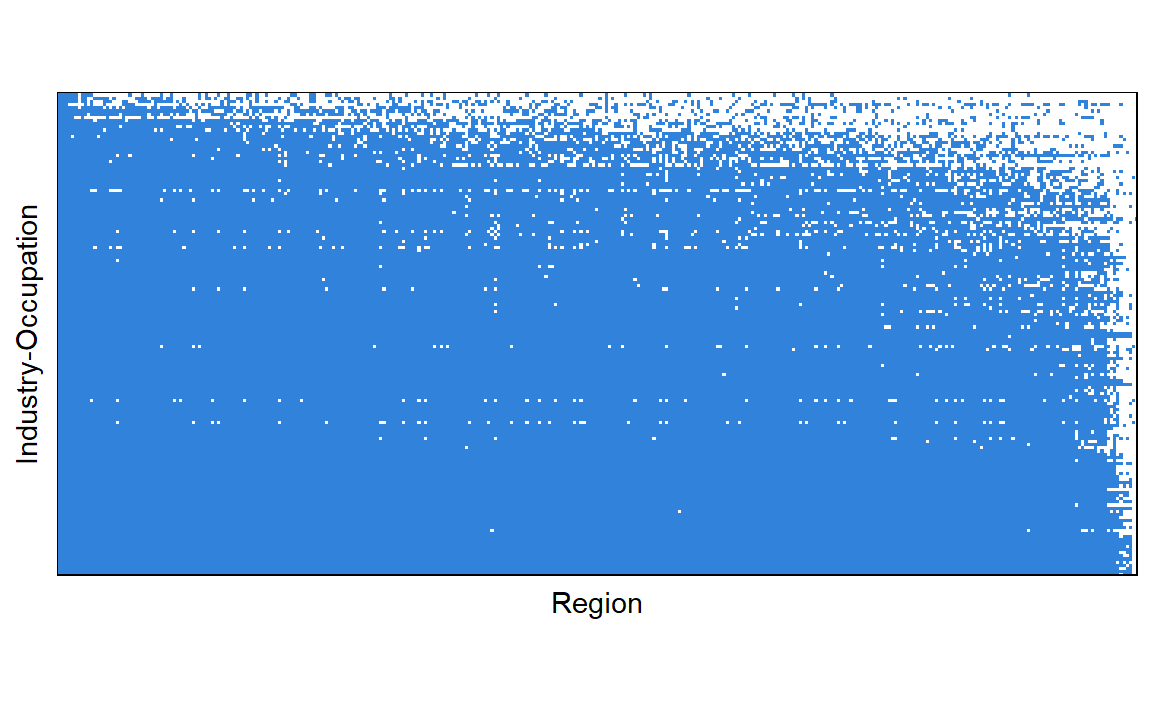
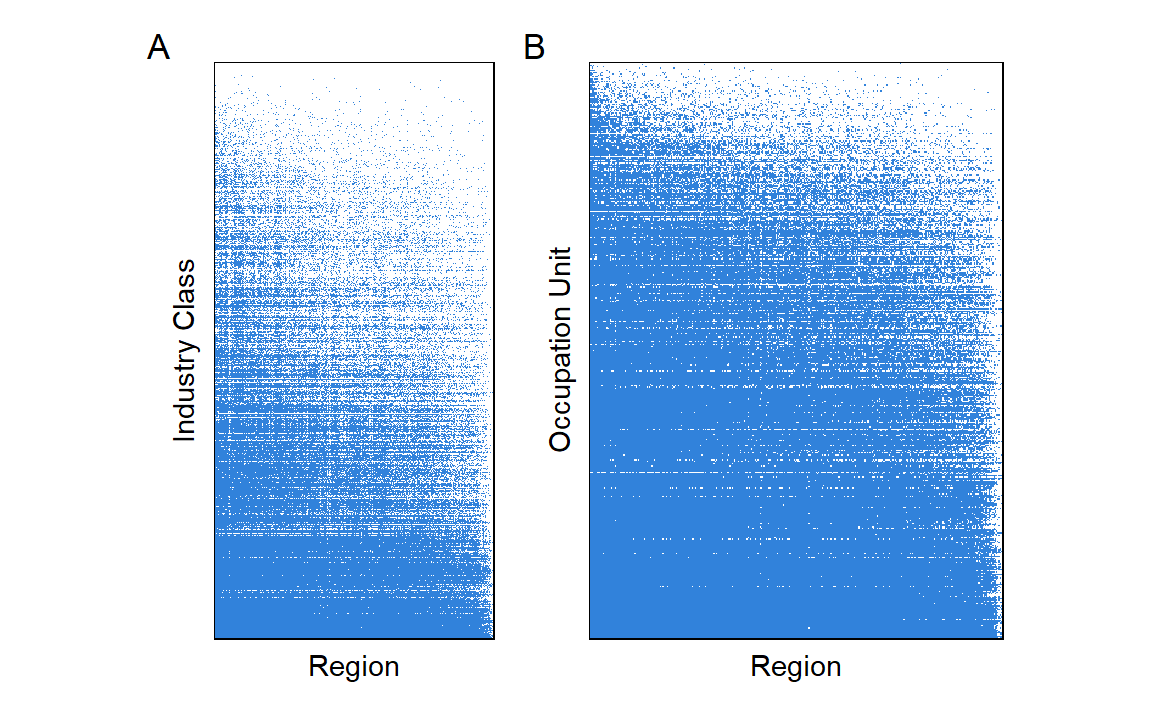
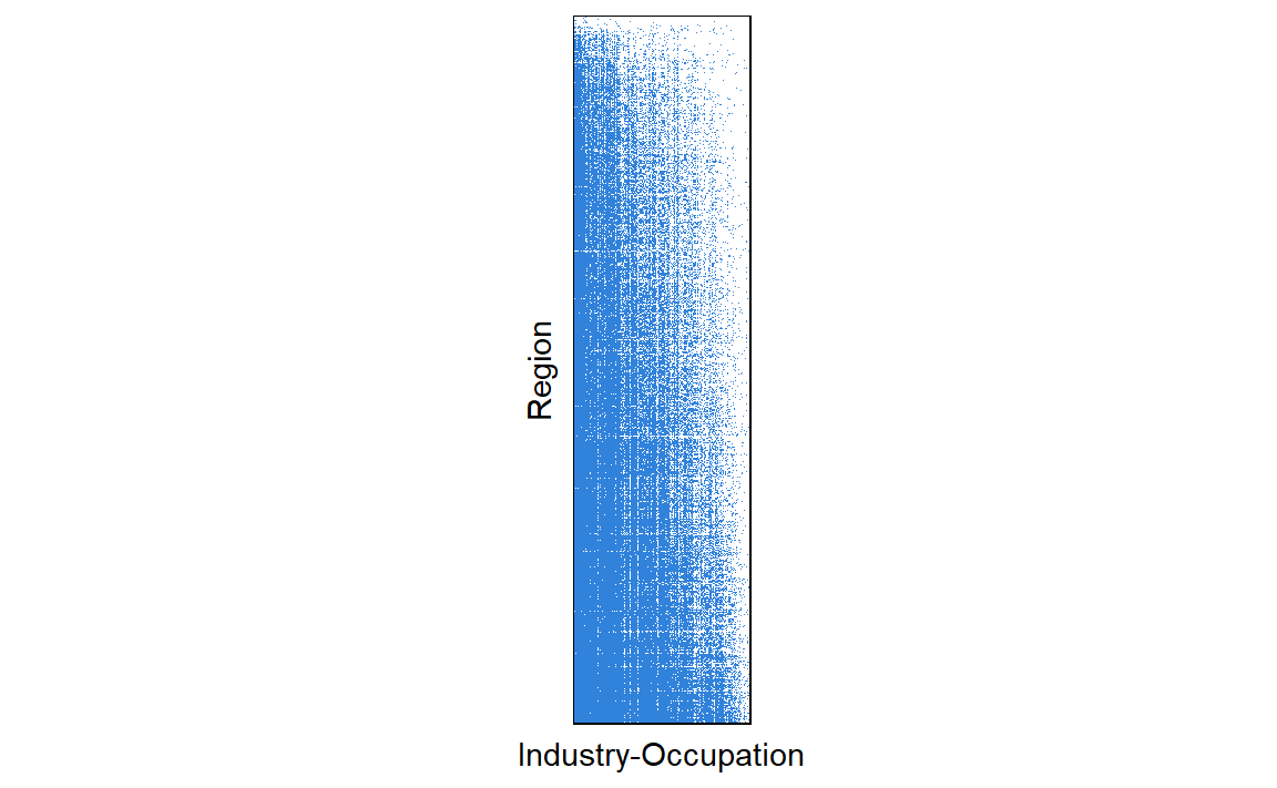
Dataset covers 340 regions and 152 industry-occupations. Figure 1 shows the presence of any level of employment within a region and industry-occupation. As can be seen, there is a high level of employment density across our data, with 88.5% of all combinations of region, industry, and occupation.
Figure 1: Presence of employment across regions and industry-occupations.
3.2 Method
This section follows the method of Davies and Maré (2021) using correlations of employment shares rather than a location quotient method.
3.2.1 Relatedness
Activities are related based on the weighted correlation between the local activity share of employment, weighted by each regions share of total employment.
Divide the weighted covariance by the city share-weighted standard deviations of the local activity shares to get the weighted correlation.
Map the correlation to the interval \([0,1]\) such that:
\[
r_{aa} = \frac{1}{2}(cor(a_i, a_j) + 1)
\]
City relatedness is calculated symmetrically such that:
\[
r_{cc} = \frac{1}{2}(cor(c_i, c_j) + 1)
\]
3.2.2 Complexity
Activity complexity is defined by the second eigenvector of the matrix \(r_{aa}\) and city complexity is defined by the second eigenvector of the matrix \(r_{cc}\). The sign of activity complexity is set such that it is positively correlated with the weighted mean size of cities that contain activity \(a\), and the sign of city complexity is set such that it is positively correlated with the local share-weighted mean complexity of activities in city \(c\)
In [3]:
# function to calculate complexity from a region * activity matrix mcomplexity_nz <-function(m, base_data) { activity_share <- m /rowSums(m) national_share_employment <-rowSums(m) /sum(m) region_name <-colnames(base_data)[1] activity_name <-colnames(base_data)[2]# Relatedness of activities is the weighted covariance between the local share vectors for activities i and j, # weighted by each regions share of total employment. r_aa <-0.5*(cov.wt(x = activity_share, wt = national_share_employment, cor =TRUE)$cor +1)#Complexity of activity a is the element a of the standardized second eigenvector of the row-standardized relatedness matrix r. complexity <-list() complexity$activity <-Re(eigen(r_aa/rowSums(r_aa))$vector[,2]) complexity$activity <- (complexity$activity -mean(complexity$activity ))/sd(complexity$activity)names(complexity$activity) <-colnames(m)#Complexity is positively correlated with the weighted mean size of cities that contain activity a wmsc <-colSums(m/colSums(m)*rowSums(m))if (cor(complexity$activity , wmsc) <0) { complexity$activity =-1*complexity$activity } else complexity$activity = complexity$activity message(glue::glue("most complex activity: {names(complexity$activity[complexity$activity == max(complexity$activity)])}")) # Relatedness of cities is symmetric to activities. city_share <-t(m /rowSums(m)) national_share_activity <-colSums(m)/sum(m) r_cc <-0.5*(cov.wt(x = city_share, wt = national_share_activity, cor =TRUE)$cor +1) complexity$city <-Re(eigen(r_cc/rowSums(r_cc))$vector[,2]) complexity$city <- (complexity$city-mean(complexity$city))/sd(complexity$city)names(complexity$city) <-rownames(m)#City complexity is positively correlated with the local share weighted mean complexity of activities in city c. wmc <-rowSums(m/colSums(m)*complexity$activity)if (cor(complexity$city, wmc) <0|| complexity$city["Brisbane Inner"] <0) { complexity$city =-1* complexity$city } else complexity$city = complexity$citymessage(glue::glue("most complex city: {names(complexity$city[complexity$city == max(complexity$city)])}")) df.complexity <-inner_join(base_data, enframe(complexity$city, name = region_name, value ="city_complexity")) |>inner_join(enframe(complexity$activity, name = activity_name, value ="activity_complexity"))return(df.complexity)}
most complex activity: Professional, Scientific and Technical Services (Professionals)
most complex city: Brisbane Inner
Joining with `by = join_by(sa3)`
Joining with `by = join_by(industry_occupation)`
complexity$indp_occp_rca <-calculate_complexity(industry_occupation_sa3, region ="sa3",product ="industry_occupation",value ="count", year =2021) |>select(sa3, industry_occupation, count, city_complexity = country_complexity_index, activity_complexity = product_complexity_index)
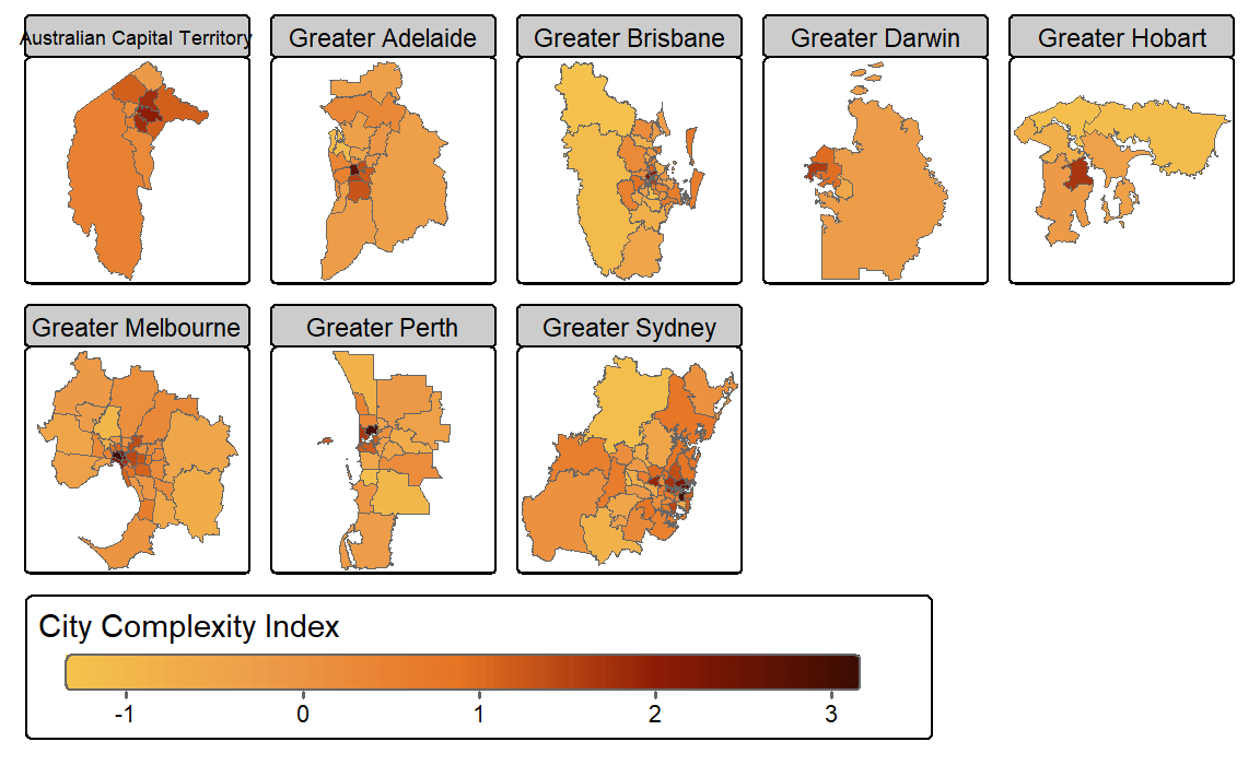
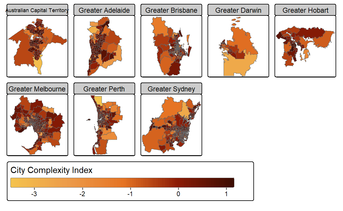
Figure 2 shows the regional complexity of SA3 regions in Australian Greater Capital City Areas based on 2021 Census data. Complexity is highest in capital cities and surrounding regions.
In [5]:
complexity_map <-function(data, layer) { data <- data |>pluck(layer) |>distinct(sa3, city_complexity) |>left_join(sa3, by =c("sa3"="sa3_name_2021")) |>st_as_sf() data |>filter(str_detect(gcc_name_2021, "Australian Capital Territory|Greater")) |>tm_shape() +tm_polygons(fill ="city_complexity",fill.scale =tm_scale_continuous(values ="greek", ),fill.legend =tm_legend(title ="City Complexity Index",orientation ="landscape")) +tm_facets("gcc_name_2021") +tm_place_legends_bottom() }complexity_map(complexity, "indp_occp")
Figure 2: Complexity of Australian Greater Capital City Areas
[plot mode] fit legend/component: Some legend items or map compoments do not fit well, and are therefore rescaled. Set the tmap option 'component.autoscale' to FALSE to disable rescaling.
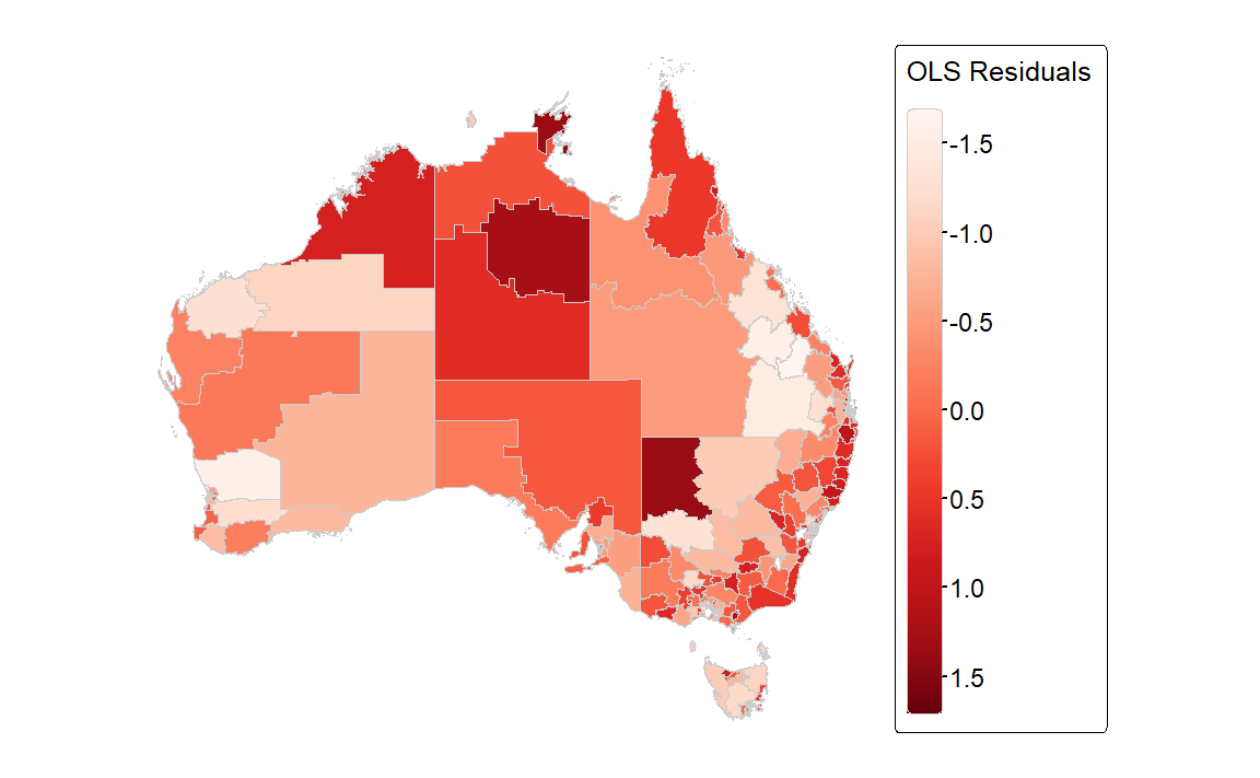
Figure 3: Residuals from linear regression
The residuals from the linear regression are shown in Figure 3 which also shows that the distribution of the residuals appears non-random.
In [10]:
moran.plot(as.numeric(scale(complexity.reg$city_complexity)),listw = lw,xlab ="City Complexity",ylab ="Neighbours City Complexity")
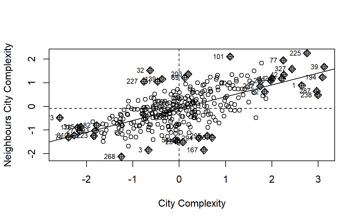
Figure 4: Moran Scatterplot for City Complexity in Australia
The correlation between complexity and lagged complexity is shown in Figure 4 which also shows a dependency. Finally, we observe a global Moran’s I of 0.498499 with a p.value of 0. As such, the data appear to be spatially autocorrelated, so a lagged AR or lagged error model should be estimated instead.
complexity$indp4 <-calculate_complexity(industry_sa3, region ="sa3", product ="indp", value ="count", year =2021) |>mutate(product ="indp4")complexity$occp4 <-calculate_complexity(occupation_sa3, region ="sa3", product ="occp", value ="count", year =2021) |>mutate(product ="occp4")
Employment density is much sparser when using 4-digit industry of employment data. Only 48 of the industry class-region combinations contain any level of employment.
In [15]:
library(patchwork)
Warning: package 'patchwork' was built under R version 4.4.1
most complex activity: Human Resource Managers
most complex city: North Sydney - Mosman
Joining with `by = join_by(sa3)`Joining with `by = join_by(occp)`
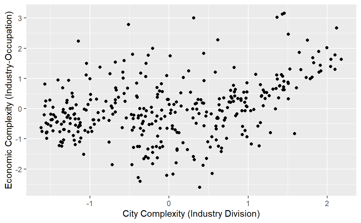
full_join(distinct(complexity$indp4, sa3, city_complexity),distinct(complexity$indp_occp, sa3, city_complexity), by ="sa3") |>ggplot(aes(x = city_complexity.x, y = city_complexity.y)) +geom_point() +labs(x ="City Complexity (Industry Division)", y ="Economic Complexity (Industry-Occupation)")
Following Mealy and Teytelboym (2022) analysis of green economic complexity, we can apply an advanced manufacturing lens to determine advanced manufacturing complexities.
In [18]:
#|am <- tibble::tribble(~indp, ~description,1811L, "Industrial gas manufacturing",1812L, "Basic organic chemical manufacturing",1813L, "Basic inorganic chemical manufacturing",1821L, "Synthetic resin and synthetic rubber manufacturing",1829L, "Other basic polymer manufacturing",1831L, "Fertiliser manufacturing",1832L, "Pesticide manufacturing",1841L, "Human pharmaceutical and medicinal product manufacturing",1842L, "Veterinary pharmaceutical and medicinal product manufacturing",1851L, "Cleaning compound manufacturing",1852L, "Cosmetic and toiletry preparation manufacturing",1891L, "Photographic chemical product manufacturing",1892L, "Explosive manufacturing",1899L, "Other basic chemical product manufacturing n.e.c.",2311L, "Motor vehicle manufacturing",2312L, "Motor vehicle body and trailer manufacturing",2313L, "Automotive electrical component manufacturing",2319L, "Other motor vehicle parts manufacturing",2391L, "Shipbuilding and repair services",2392L, "Boatbuilding and repair services",2393L, "Railway rolling stock manufacturing and repair services",2394L, "Aircraft manufacturing and repair services",2399L, "Other transport equipment manufacturing n.e.c.",2411L, "Photographic, optical and ophthalmic equipment manufacturing",2412L, "Medical and surgical equipment manufacturing",2419L, "Other professional and scientific equipment manufacturing",2421L, "Computer and electronic office equipment manufacturing",2422L, "Communication equipment manufacturing",2429L, "Other electronic equipment manufacturing",2431L, "Electric cable and wire manufacturing",2432L, "Electric lighting equipment manufacturing",2439L, "Other electrical equipment manufacturing",2441L, "Whiteware appliance manufacturing",2449L, "Other domestic appliance manufacturing",2451L, "Pump and compressor manufacturing",2452L, "Fixed space heating, cooling and ventilation equipment manufacturing",2461L, "Agricultural machinery and equipment manufacturing",2462L, "Mining and construction machinery manufacturing",2463L, "Machine tool parts and parts manufacturing",2469L, "Other specialised machinery and equipment manufacturing",2491L, "Lifting and handling equipment manufacturing",2499L, "Other machinery and equipment manufacturing" ) |>mutate(indp =as.character(indp))
In [19]:
amci <-calculate_complexity(industry_sa3, region ="sa3", product ="indp", value ="count", year =2021) |>mutate(m =as.numeric(rca >=1),is_am =as.numeric(indp %in% am$indp),pci = scales::rescale(product_complexity_index, to =c(0, 1)),p = m * is_am) |>group_by(sa3) |>summarise(amci =sum(pci * p),amp =sum((1-p)*density*pci)/sum(1-p),amce =sum(count*is_am)) |>mutate(across(c(amci, amp), ~ (.x -mean(.x))/sd(.x)))complexity.reg <- complexity.reg |>inner_join(amci)
Adam, Antonis, Antonios Garas, Marina-Selini Katsaiti, and Athanasios Lapatinas. 2023. “Economic Complexity and Jobs: An Empirical Analysis.”Economics of Innovation and New Technology 32 (1): 25–52. https://doi.org/10.1080/10438599.2020.1859751.
Balland, Pierre-Alexandre, and Ron Boschma. 2021. “Mapping the Potentials of Regions in Europe to Contribute to New Knowledge Production in Industry 4.0 Technologies.”Regional Studies 55 (10-11): 1652–66. https://doi.org/10.1080/00343404.2021.1900557.
Chávez, Juan Carlos, Marco T. Mosqueda, and Manuel Gómez-Zaldívar. 2017. “Economic Complexity and Regional Growth Performance: Evidence from the Mexican Economy.”Review of Regional Studies 47 (2): 201–19. https://doi.org/10.52324/001c.8023.
Fritz, Benedikt S. L., and Robert A. Manduca. 2021. “The Economic Complexity of US Metropolitan Areas.”Regional Studies 55 (7): 1299–1310. https://doi.org/10.1080/00343404.2021.1884215.
Gao, Jian, and Tao Zhou. 2018. “Quantifying China’s Regional Economic Complexity.”Physica A: Statistical Mechanics and Its Applications 492: 1591–1603. https://doi.org/https://doi.org/10.1016/j.physa.2017.11.084.
Guevara, Miguel R., Dominik Hartmann, Manuel Aristarán, Marcelo Mendoza, and César A. Hidalgo. 2016. “The Research Space: Using Career Paths to Predict the Evolution of the Research Output of Individuals, Institutions, and Nations.”Scientometrics 109 (3): 1695–1709. https://doi.org/10.1007/s11192-016-2125-9.
Hartmann, Dominik, Miguel R. Guevara, Cristian Jara-Figueroa, Manuel Aristarán, and César A. Hidalgo. 2017. “Linking Economic Complexity, Institutions, and Income Inequality.”World Development 93 (May): 75–93. https://doi.org/10.1016/j.worlddev.2016.12.020.
Hidalgo, C. A., B. Klinger, A.-L. Barabaśi, and R. Hausmann. 2007. “The Product Space Conditions the Development of Nations.”Science 317 (5837): 482–87. https://doi.org/10.1126/science.1144581.
Hidalgo, César A., and Ricardo Hausmann. 2009. “The Building Blocks of Economic Complexity.”Proceedings of the National Academy of Sciences 106 (26): 10570–75. https://doi.org/10.1073/pnas.0900943106.
Kogler, Dieter F., David L. Rigby, and Isaac Tucker. 2013. “Mapping Knowledge Space and Technological Relatedness in US Cities.”European Planning Studies 21 (9): 1374–91. https://doi.org/10.1080/09654313.2012.755832.
Muneepeerakul, Rachata, José Lobo, Shade T. Shutters, Andrés Goméz-Liévano, and Murad R. Qubbaj. 2013. “Urban Economies and Occupation Space: Can They Get “There” from “Here”?” Edited by César A. Hidalgo. PLoS ONE 8 (9): e73676. https://doi.org/10.1371/journal.pone.0073676.
Neffke, Frank, and Martin Henning. 2012. “Skill Relatedness and Firm Diversification.”Strategic Management Journal 34 (3): 297–316. https://doi.org/10.1002/smj.2014.
Reynolds, Christian, Manju Agrawal, Ivan Lee, Chen Zhan, Jiuyong Li, Phillip Taylor, Tim Mares, Julian Morison, Nicholas Angelakis, and Göran Roos. 2018. “A Sub-National Economic Complexity Analysis of Australia’s States and Territories.”Regional Studies 52 (5): 715–26. https://doi.org/10.1080/00343404.2017.1283012.